


Rate Monotonic Scheduling and Schedulability Analysis in RTOS
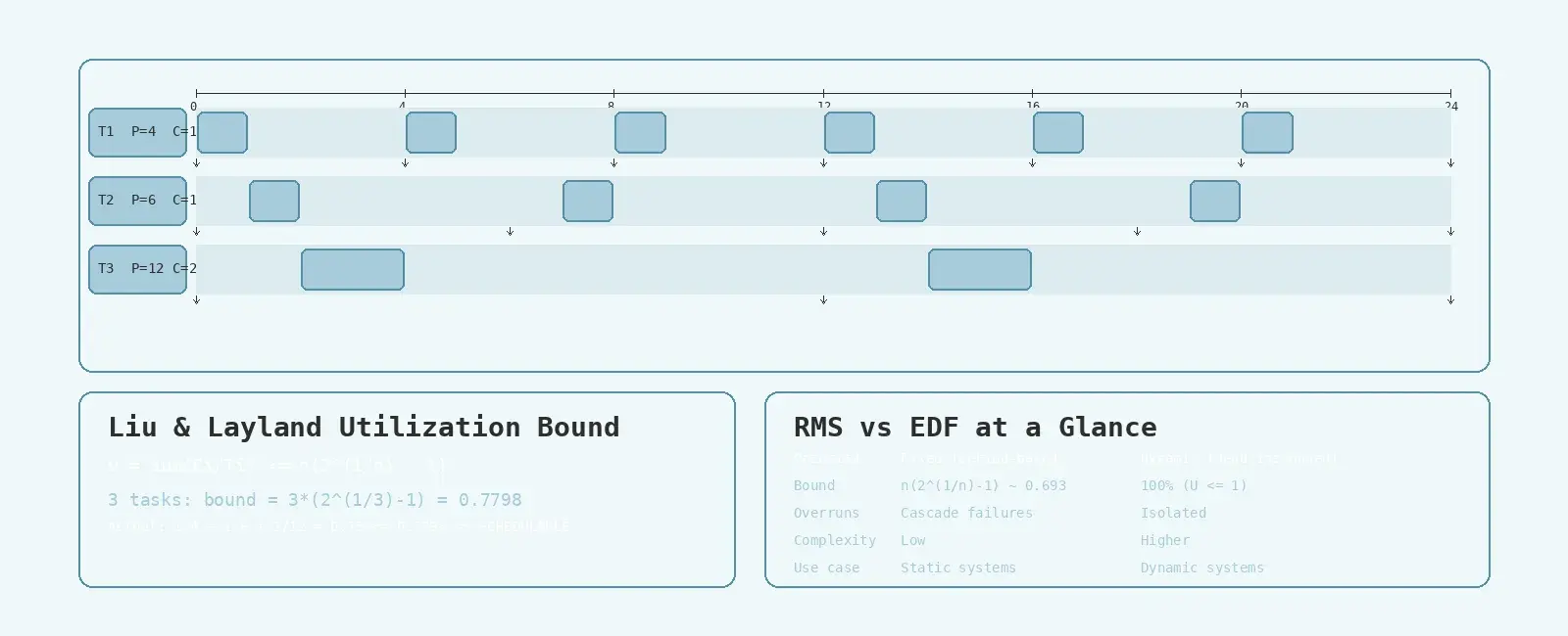
Table Of Contents
Every real-time system has deadlines. A motor controller must complete its control loop within a millisecond. A communication stack must respond to incoming frames before the buffer overflows. Missing a deadline in a hard real-time system is not a performance hiccup — it is a system failure.
But how do you prove that a set of tasks will always meet their deadlines? You cannot test your way to this guarantee; testing covers specific scenarios, not every possible combination of task arrivals. The answer is schedulability analysis — a mathematical framework that lets you verify timing correctness at design time. The most widely used approach for fixed-priority systems is Rate Monotonic Scheduling (RMS), and its companion, the Liu & Layland utilization bound.
This article covers the theory behind RMS, how to apply the utilization bound test, its limitations, and how it compares to the more flexible Earliest Deadline First (EDF) approach.
The Task Model
Real-time scheduling theory models each periodic task as a tuple (C, T, D) where:
- C = Worst-case execution time (WCET)
- T = Period (how often the task releases)
- D = Deadline (relative to release; for implicit-deadline systems, D = T)
A task releases a new job every T time units. Each job must complete C units of computation before the deadline D. The system is schedulable if every job of every task completes before its deadline, under all possible release patterns.
+=======================================================================+| PERIODIC TASK MODEL || || Task Ti = (Ci, Ti, Di) || || Time ----|----|----|----|----|----|----|----|----> || ^ ^ ^ ^ ^ ^ ^ ^ || | | | | | | | | || release release release release release || |<--C-->| || | deadline D (must finish here) || || Utilization: Ui = Ci / Ti || Total load: U = sum(Ci/Ti) for all tasks |+=======================================================================+
The utilization of a single task is Ui = Ci/Ti — the fraction of CPU time it consumes. The total system utilization U is the sum of all individual utilizations. If U > 1.0, the system is trivially unschedulable (the tasks demand more CPU time than exists). But U <= 1.0 does not guarantee schedulability — it is necessary but not sufficient.
Rate Monotonic Priority Assignment
Rate Monotonic Scheduling assigns priorities based on period: shorter period = higher priority. A task that runs every 2ms gets higher priority than a task that runs every 10ms. This is a fixed-priority scheme — priorities are assigned at design time and never change.
The intuition is simple: tasks with tighter timing constraints (shorter periods) should preempt tasks with looser constraints. A task that must finish every 2ms cannot afford to be delayed by a task that has 10ms to complete.
+=======================================================================+| RATE MONOTONIC PRIORITY ASSIGNMENT || || Task Period Priority Reason || ---- ------ -------- ------ || T1 4ms HIGHEST Shortest period || T2 6ms MEDIUM Medium period || T3 12ms LOWEST Longest period || || Rule: Shorter period -> Higher priority || (Static -- priorities never change at runtime) |+=======================================================================+
RMS is optimal among all fixed-priority assignment schemes for implicit-deadline systems (D = T): if such a task set is schedulable under any fixed-priority assignment, it is also schedulable under RMS. This makes it the natural choice for static RTOS configurations where priorities are set at compile time.
The Liu & Layland Utilization Bound
In their seminal 1973 paper, Liu and Layland proved a remarkable result: a set of n implicit-deadline periodic tasks is guaranteed schedulable under RMS if:
U = sum(Ci/Ti) <= n * (2^(1/n) - 1)
This bound depends only on the number of tasks, not on their specific periods or execution times. (Note: If task periods are harmonic—meaning every period is an exact integer multiple of all shorter periods—the utilization bound is 1.0, or 100%.) For small n:
| Number of tasks (n) | Utilization bound |
|---|---|
| 1 | 1.0000 (100%) |
| 2 | 0.8284 (82.8%) |
| 3 | 0.7798 (78.0%) |
| 4 | 0.7568 (75.7%) |
| 5 | 0.7435 (74.3%) |
| 10 | 0.7177 (71.8%) |
| infinity | 0.6931 (69.3%) |
As n grows, the bound approaches ln(2) ~ 0.693. This means: with many tasks, RMS guarantees schedulability only up to about 69% CPU utilization. Above that, the test is inconclusive — the task set might still be schedulable, but the bound cannot prove it.
+=======================================================================+| LIU & LAYLAND BOUND: UTILIZATION vs TASK COUNT || || 1.0 |* || | * || 0.9 | * || | ** || 0.8 | ** || | ** || 0.7 | ***................................... || | (approaches ln(2) = 0.693) || 0.6 | || +----+----+----+----+----+----+----+----+----+---> || 0 2 4 6 8 10 12 14 16 18 || Number of tasks (n) || || If U <= bound: GUARANTEED schedulable || If U > bound: INCONCLUSIVE (need exact analysis) |+=======================================================================+
Worked Example
Consider three tasks on an RTOS:
- T1: C=1ms, T=4ms (control loop)
- T2: C=1ms, T=6ms (sensor polling)
- T3: C=2ms, T=12ms (data logging)
Total utilization: U = 1/4 + 1/6 + 2/12 = 0.25 + 0.1667 + 0.1667 = 0.5833
Liu & Layland bound for n=3: 3 * (2^(1/3) - 1) = 0.7798
Since 0.5833 <= 0.7798, the task set is guaranteed schedulable under RMS. No further analysis needed.
Now consider a heavier load:
- T1: C=2ms, T=4ms (U=0.50)
- T2: C=2ms, T=6ms (U=0.333)
- T3: C=3ms, T=12ms (U=0.25)
Total: U = 1.083 — trivially unschedulable (exceeds 100%).
A more interesting case:
- T1: C=1ms, T=4ms (U=0.25)
- T2: C=2ms, T=6ms (U=0.333)
- T3: C=2ms, T=12ms (U=0.167)
Total: U = 0.75 — below the 0.7798 bound, so guaranteed schedulable.
But if T3’s execution time increases to C=3ms (U=0.25), total becomes 0.833 — above the bound. The test is inconclusive. The task set might still be schedulable, but you need exact analysis (response time analysis) to find out.
Response Time Analysis: The Exact Test
When the utilization bound test is inconclusive, you can use Response Time Analysis (RTA) to get an exact answer. For each task, compute the worst-case response time R — the longest time from job release to completion.
For any task Ti, the worst-case response time occurs when it releases simultaneously with all higher-priority tasks (the critical instant). The response time is computed iteratively:
Ri = Ci + sum( ceil(Ri / Tj) * Cj ) for all higher-priority tasks j
You start with Ri = Ci and iterate until Ri converges (stops changing) or exceeds the deadline.
+=======================================================================+| RESPONSE TIME ANALYSIS PROCEDURE || || For each task Ti (from highest to lowest priority): || || 1. Start with Ri = Ci || 2. Compute interference from higher-priority tasks: || I = sum( ceil(Ri / Tj) * Cj ) for j < i || 3. New Ri = Ci + I || 4. If New Ri > Di: MISS -- task set unschedulable || 5. If New Ri == Ri: CONVERGED -- Ti is schedulable, check next task || 6. Else: Ri = New Ri, go to step 2 || || All tasks converge within deadline => SCHEDULABLE |+=======================================================================+
RTA is exact: if it says the task set is schedulable, it truly is. If it says a deadline is missed, the critical instant scenario will cause it. This makes RTA the gold standard for certification of safety-critical systems (DO-178C, ISO 26262).
RMS vs EDF: When Fixed Priorities Are Not Enough
RMS is simple and efficient — perfect for static RTOS configurations. But its 69% utilization ceiling (for many tasks) wastes CPU capacity. Earliest Deadline First (EDF) is a dynamic-priority scheduler that achieves 100% utilization: a task set is schedulable under EDF if and only if U <= 1.0.
| Property | RMS | EDF |
|---|---|---|
| Priority assignment | Fixed (period-based) | Dynamic (deadline-based) |
| Schedulability bound | n(2^(1/n)-1) ~ 0.693 | 1.0 (100%) |
| Runtime overhead | Very low | Slightly higher |
| Overrun behavior | Isolated deadline misses | Cascade failures |
| Implementation complexity | Simple | Moderate |
| Best for | Static, safety-critical | Dynamic, high-utilization |
EDF re-evaluates priorities at every scheduling point: the task with the earliest absolute deadline runs next. This requires tracking absolute deadlines and sorting the ready queue, which adds overhead. More critically, if one task overruns its execution time, EDF can cascade deadline misses across multiple tasks in unpredictable ways. RMS contains overruns: a low-priority task overrun only affects lower-priority tasks.
For most embedded RTOS deployments (FreeRTOS, Zephyr, ThreadX), fixed-priority scheduling is the default and often the only option. RMS provides a clean, analyzable framework that maps directly to the RTOS priority model.
Practical Considerations
The Liu & Layland analysis assumes:
- Independent tasks (no shared resources, no blocking)
- Implicit deadlines (D = T)
- Zero context switch overhead
- Instantaneous job release (no release jitter)
Real systems violate all of these assumptions. Shared resources introduce blocking time (handled by adding blocking terms to RTA). Context switch overhead can be modeled by inflating each task’s execution time by twice the context switch cost. Deadlines shorter than periods (constrained deadlines) require the more general Deadline Monotonic priority assignment.
Despite these limitations, the utilization bound test remains valuable as a quick sanity check during design. If your total utilization is below the bound, you have a mathematical guarantee. If it is above, you know you need deeper analysis — or a lighter workload.
Summary
Rate Monotonic Scheduling is the foundation of real-time scheduling theory and the default model for most RTOS-based embedded systems. The Liu & Layland utilization bound provides a simple, powerful test: if total CPU utilization is below n(2^(1/n)-1), your task set is guaranteed to meet all deadlines. When the bound is exceeded, Response Time Analysis gives an exact answer. For systems that need more than 69% utilization, EDF offers 100% CPU efficiency at the cost of dynamic priorities and more complex failure modes. Understanding these tradeoffs is essential for designing predictable, certifiable real-time embedded systems.
Related Reading
- Context Switching and Scheduling in RTOS - A Deep Dive — how the kernel implements preemptive scheduling
- Priority Inversion and Inheritance in RTOS — what happens when priority ordering breaks down
References
- Liu, C. L. & Layland, J. W. — “Scheduling Algorithms for Multiprogramming in a Hard-Real-Time Environment” (Journal of the ACM, vol. 20, no. 1, pp. 46-61, 1973) — the foundational paper that introduced Rate Monotonic Scheduling and proved the utilization bound theorem.
- Buttazzo, G. C. — Hard Real-Time Computing Systems: Predictable Scheduling Algorithms and Applications (4th ed., Springer, 2024) — comprehensive textbook covering RMS, EDF, response time analysis, resource access protocols, and server-based scheduling.
- Burns, A. & Wellings, A. — Real-Time Systems and Programming Languages (4th ed., Addison-Wesley, 2009) — Chapter 7 covers schedulability analysis for fixed-priority systems including the Liu & Layland bound, response time analysis, and the effects of blocking.
- Audsley, N. C., Burns, A., Richardson, M., Tindell, K., & Wellings, A. J. — “Applying New Scheduling Theory to Static Priority Pre-emptive Scheduling” (Software Engineering Journal, vol. 8, no. 5, pp. 284-292, 1993) — extended the Liu & Layland analysis to handle arbitrary deadlines, context switch overhead, and other practical factors.
Related Posts
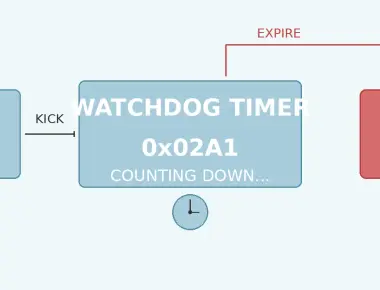
Watchdog Timers in Embedded Systems
June 17, 2026
3 min
RTOS Performance Profiling and Optimization Techniques
June 10, 2026
3 min
Low-Power Design Patterns for RTOS-Based Embedded Systems
June 07, 2026
4 min
RTOS Task Notifications vs Queues - When to Use Each in FreeRTOS
June 06, 2026
3 min
Stack Overflow Detection and Monitoring in RTOS
June 05, 2026
4 min
Quick Links
Legal Stuff